Continuing the data structures, in this article I will write about graphs. These structures can be used in a big variety of applications. For implementation I will use an adjacency list approach, but in the introduction I also talk about the adjacency matrix version. Apart from the implementation I write (and talk) about the theory and real life usages of graphs.

Theory and basics

As I already mentioned in the introduction, graphs are used in many-many places – even if we don’t know it directly. The thing is, graphs can represent almost anything because its nature. Graph contains nodes and edges which can be interpreted as the task requires it to be. For example edges can represent simple bool/false connections like personal connections on Facebook or on Instagram. It can also represent cities and connecting roads in case of Google Maps; or it can represent a full game level where the player can move on a grid and there are other good examples. Keep in mind that there are plenty of other graph algorithms in the “graph world”, in this article I only mention the well known and most important ones.

Types

Basically there are four different ways how we can use graphs. A graph in the same time can not be directed and undirected (it’s a contradiction). However, in the same time a graph can be directed or undirected and weighted or unweighted.

So, the possible scenarios:

• directed and weighted
• directed and unweighted
• undirected and weighted
• undirected and unweighted

Directed

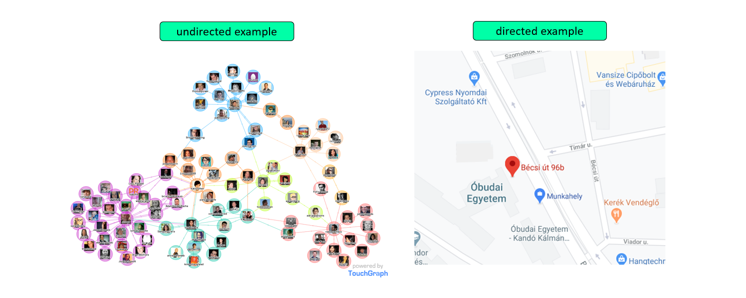
If a graph is directed, it means that from one node to the other you can only go in one direction which is where the arrow points. Of course, if the arrow points back and forth, it means that you can go from A to B, and vica versa. If there is no arrow at all (it means there is no edge between A and B) then it means there is no connection between them.

Good example if we think about roads and cross sections. Roads are the edges and cross sections are the nodes. There is no theoretical limit how many roads can connect into one cross section (think about a huge roundabout). In this case, the edges (which are directed) can be interpreted as one-way or two-way roads.

Undirected

If a graph is undirected, it means that there is no restriction if you can go from A to B or from B to A. Basically we can say that an undirected graph is a directed graph where all the edges are directed in both ways.

For example when you want to represent people connections (like Facebook friends) it automatically means that person A and person B are connected, so there is no need for any directed edges between them.

Weighted

Edges can be used with weights added to them. In this case it can represent any kind of “cost function”. Imagine something like the first example, when we have roads and cities. The roads connect the cities. These roads – in real life as well – have length which me measure in kilometers or miles. In a weighted graph we can use the length of each road as a weight added to the given edge in the graph.

Unweighted

If a graph is unweighted it simply means that there is no additional information about the edge between A and B.

Representation

There are two ways for graph representation. Adjacency list is good if we have a frequently changing graph structure, because in this case we need a dynamic data structure inside which we can add/remove items. Of course, using any kind of list (like linked list) has it’s downsides. If we have a fixed graph where barely no nodes are inserted then an adjacency matrix can be used for representation. As the name suggests matrix (or two dimensional array) is used for the inside structure with all of its upsides. So basically there is no best way – it depends on what you need to do.

C# code example

The adjacency list version of a generic graph data structure can be seen on the code below. It’s worth mentioning that inserting a new item into the graph can be done in two parts: a) inserting the node itself, b) connecting the node with other nodes (adding edges between node A and B). Using adjacency list we simply use a list of lists approach – which is equivalent to a jagged array.

1
2
3
4
5
6
7
8
9
10
11
12
13
14
15
16
17
18
19
20
class Graph<T>
{
    List<List<T>> adjacencyList = new List<List<T>>();
    List<T> content = new List<T>();

    public void AddNode(T node)
    {
        content.Add(node);
        adjacencyList.Add(new List<T>());
    }

    public void AddEdge(T from, T to)
    {
        int indexFrom = content.IndexOf(from);
        int indexTo = content.IndexOf(to);

        adjacencyList[indexFrom].Add(content[indexTo]);
        adjacencyList[indexTo].Add(content[indexFrom]);
    }
}

Traversals

Graph traversals are not as straightforward as it’s in case of a binary search tree for example. The thing is, where should we start the traversal? There is no head in a graph, which could be the starting point. So for this, we will have different traversals for different scenarios. In each case we must select the starting point.

DFS & BFS

DFS stands for Depth First Search, which is a well-known traversal algorithm, just like BFS which stands for Breadth First Search.

DFS starts at a selected node and explores as far as possible along each branch before backtracking. So basically it goes to the deepest in the graph, and then if there is no other options it starts stepping back.

Compared to this BFS also starts at a selected node and then explores all of the neighbor nodes at the present depth prior to moving on to the nodes at the next depth level. So instead of going to the deepest part instantly, it travels like a wave-front on the water and processing each node at the same depth level.

Important detail:

• DFS uses stack to store the items which will be processed later, so the backtracking part makes sense, but the usage of the stack can be evaded because the recursive function calls basically represent a stack-like sequence. (On the video below this is explained in detail.)
• BFS uses queue to store the items which will be processed later, this usage can not be aveded.

DFS and BFS traversals, alongside with the theory can be watched in this video:

Dijkstra

Dijsktra is the most famous, well-known (shortest) path finding algorithm. With the help of this we can determine the shortest route between point A (which is the starting point) and any other point (which we can select later).

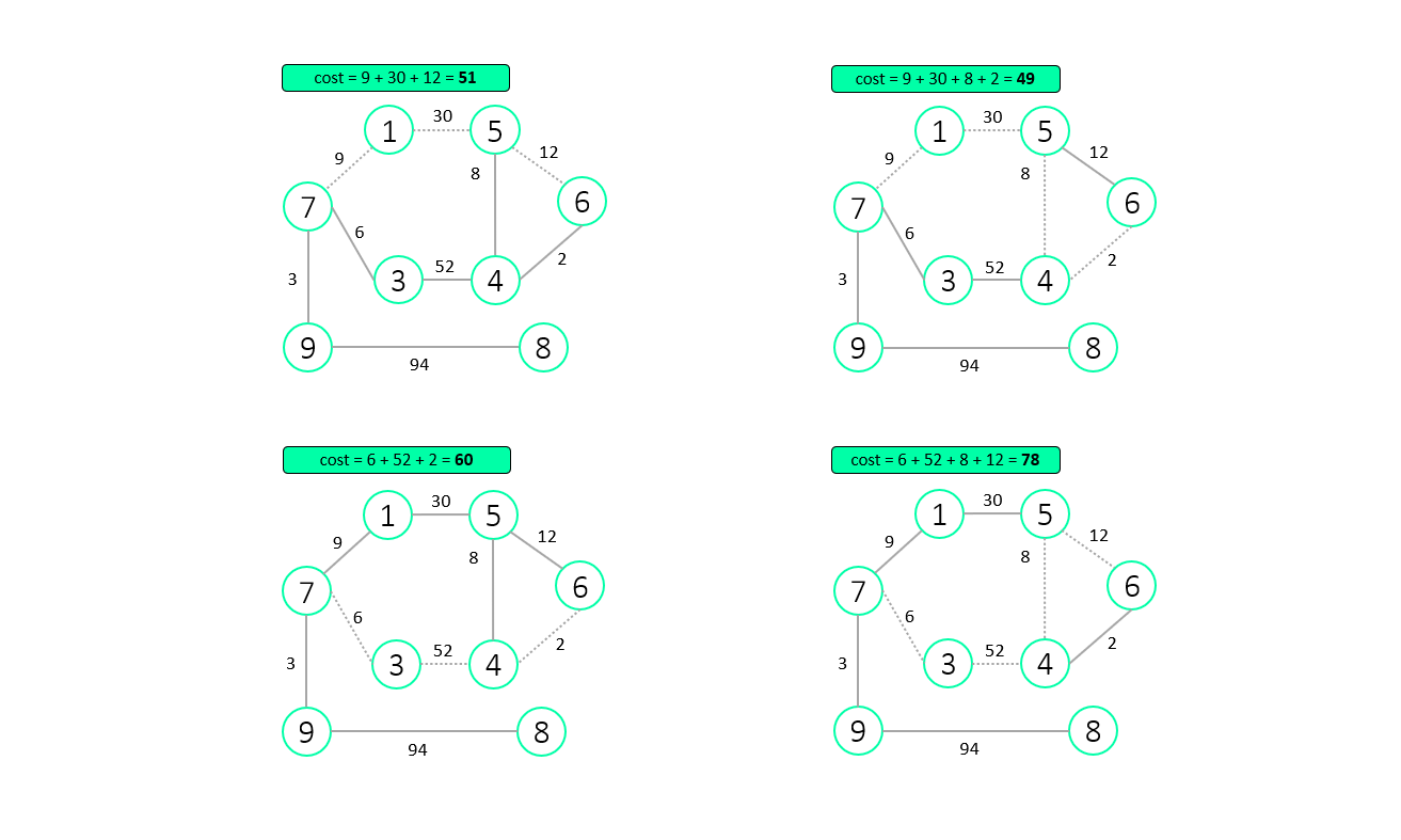
On the example below the starting point was node (7) and the finish point was node (6). All the possible routes between them are represented as different scenarios, with the full cost of each. From this it’s obvious that the second scenario (top right) is the best route between (7) and (6) nodes, meaning that it has the lowest cost.

Kruskal

In short, Kruskal’s algorithm can be used to determine the minimum spanning tree of the graph. This is good for us if we need to have a sub-graph where all the nodes are selected but only with the less costly edges. In more precise terms: Given a connected and undirected graph, a spanning tree of that graph is a subgraph that is a tree and connects all the vertices together. A single graph can have many different spanning trees. A minimum spanning tree (MST) or minimum weight spanning tree for a weighted, connected and undirected graph is a spanning tree with weight less than or equal to the weight of every other spanning tree. The weight of a spanning tree is the sum of weights given to each edge of the spanning tree.

A good example where we can use spanning trees as a real life application is network design.